Wireless Propagation Scenario

Create a wireless propagation scenario where the transmitter and receiver are 100*(your roll number) m apart. Omnidirectional antennas are used at transmitter and receiver. The gain of the antennas is 0.5 dB. The transmit power is 1 mW. The operating frequency is 14*(your roll number) GHz. Use Matlab for the simulations.

a) What is the received power and path loss when one line-of-sight and 5 reflected paths are present? The power of the reflected paths can be taken as the negative exponential of the line-of-sight path power as [exp(-LOS) exp(-2*LOS) exp(-3*LOS) exp(-4*LOS) exp(-5*LOS)].

Solution:

Distance of transmitter and receiver is = 100 * roll no = 100 * 24 = 2400m

Gain of Antenna = 0.5dB

Transmit Power = P_T = 1mW = 1e-3 W

Operating frequency = f = 14 * roll no = 14 * 24 = 336GHz

Part a:

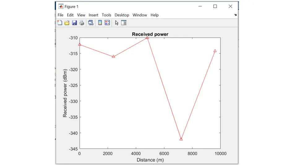
Received power and path loss when one line-of-sight and 5 reflected paths are present is calculated in the following MATLAB code:

Calculating Receive power:

% Calculating Receive power:
function [d,P_R,P_T] = Receive_power_single(P_T,G_T,G_R,lam)

% Receive power calculated for line of sight path
m = 100*24        			             %distance = 100 * roll on
gain_p = 1;         			             %line of sight path gain is 1
los = (P_T.*G_T.*G_R.*lam.*lam.*gain_p)./((4.*pi.*m).^2)

d = 1:m:12000               		% Distance in meters with difference of 100*roll no
P_R = zeros(5,1);            		% Received power
alp = rand(5,1).*[1e-1*los 1e-2*los 1e-3*los 1e-4*los 1e-5*los];    % Random gain of path
d_ind = d.*rand(5,1);        		                     % Random distance of the path

% total receive power of reflected path
for i = 1:5    				        %take loop from 1 to 5 for reflected paths
         P_R(i) = sum((P_T.*G_T.*G_R.*lam.*lam.*alp(i,:))./((4.*pi.*d_ind(i,:)).^2))
end

% total receive power (line of sight path + Reflected path):
total = los + P_R(i);

figure
plot(d,10*log10(P_R), 'r^-')
xlabel('Distance (m)')
ylabel('Received power (dBm)')
title('Received power')
end

Now Path loss function is:

Calculating Path Loss:

%Calculating Path Loss:
function path_loss_calculation
clear all 
close all
P_T = 1e-3;                                          % Transmit power
G_T  = 0.5;                                          % Transmit gain of antenna
G_R = G_T;                                           % Receive gain of antenna
lam = 3e8/336e9;                                     % Wavelength

[d,P_R,P_T] = Receive_power_single(P_T,G_T,G_R,lam)

PL = 0;
PL = P_T./P_R;                                        % Path loss

d0 = 1;                                               % Reference distance
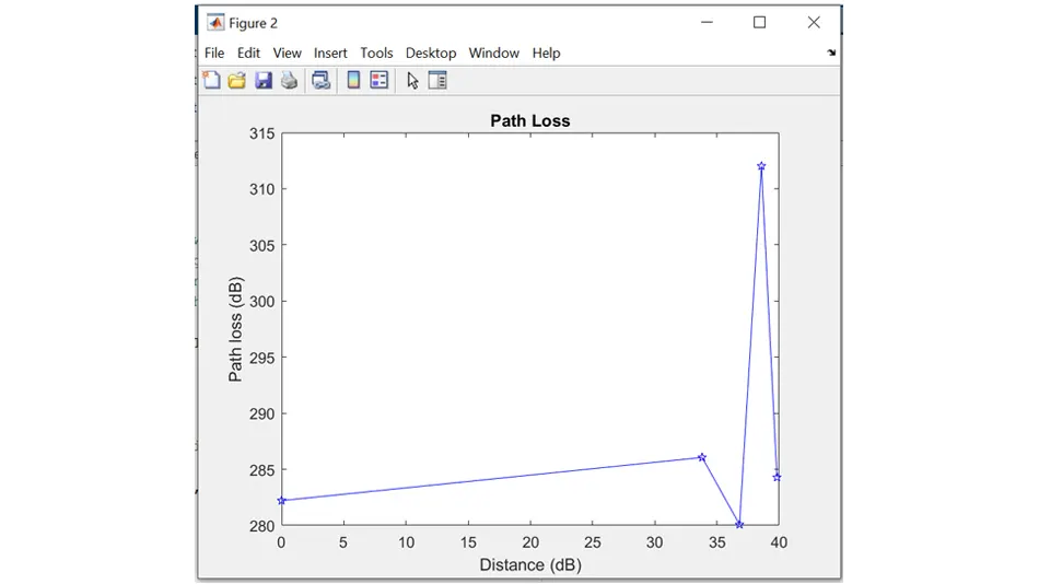
figure
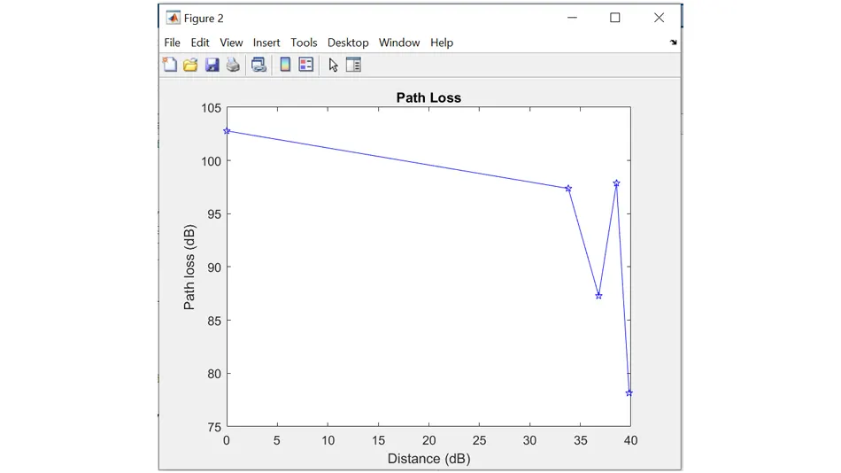
plot(10*log10(d/d0),10*log10(abs(PL)), 'bp-')
xlabel('Distance (dB)')
ylabel('Path loss (dB)')
title('Path Loss')


p = 0;
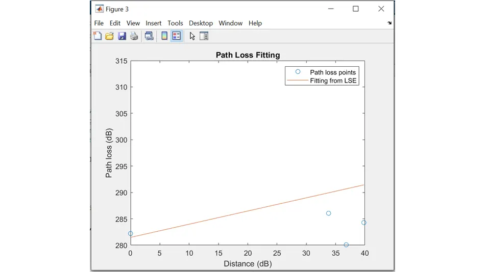
p = polyfit(10*log10(d.'),10*log10(abs(PL)),1);
y1 = polyval(p,10*log10(d));

figure
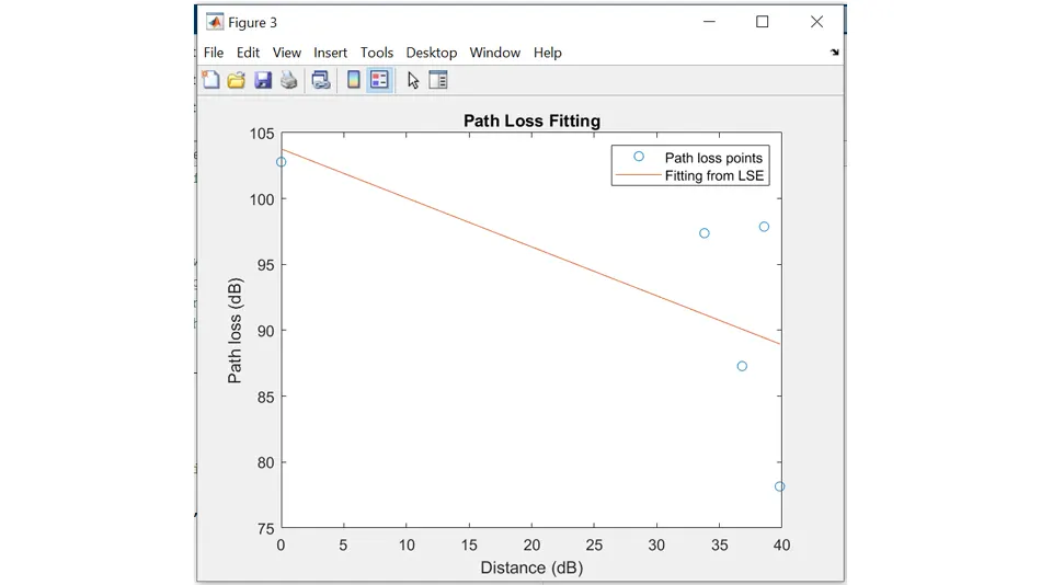
plot(10*log10(d.'),10*log10(abs(PL)),'o')
hold on
plot(10*log10(d.'),y1)
xlabel('Distance (dB)')
ylabel('Path loss (dB)')
legend('Path loss points', 'Fitting from LSE')
title('Path Loss Fitting')
hold off
abs(p(1))

Output Windows:

The figures of the above code are as follows:

Now Path loss and path loss fitting is:

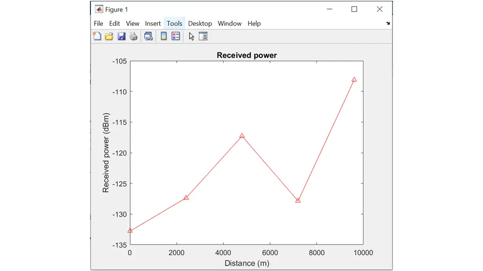
Part b: What is the received power and path loss when no line-of-sight is present and only 5 reflected paths are present? The power of the reflected paths can be taken as the negative exponential of [1 2 3 4 5].

Received power and path loss when no line-of-sight is present and only 5 reflected paths are present are calculated as following code:

Calculating Receive power of without line of sight:

% Calculating Receive power of without line of sight:
function [d,P_R,P_T] = Receive_power_single1(P_T,G_T,G_R,lam)

d = 1:2400:12000                                                  % Distance in meters
P_R = zeros(5,1);                                                 % Received power
alp = rand(5,1).*[1e-1 1e-2 1e-3 1e-4 1e-5];                      % Random gain of path
d_ind = d.*rand(5,1);                                      % Random distance of the path

for i = 1:5
                P_R(i) = sum((P_T.*G_T.*G_R.*lam.*lam.*alp(i,:))./((4.*pi.*d_ind(i,:)).^2));
end

figure
plot(d,10*log10(P_R), 'r^-')
xlabel('Distance (m)')
ylabel('Received power (dBm)')
title('Received power')
end

Now path loss is:

Calculating Path Loss with no line of sight:

%Calculating Path Loss with no line of sight:
function path_loss1
clear all 
close all
P_T = 1e-3;                                             % Transmit power
G_T  = 0.5;                                             % Transmit gain of antenna
G_R = G_T;                                              % Receive gain of antenna
lam = 3e8/336e9;                                        % Wavelength

[d,P_R,P_T] = Receive_power_single1(P_T,G_T,G_R,lam)

PL = 0;
PL = P_T./P_R;                                          % Path loss

d0 = 1;                                                 % Reference distance
figure
plot(10*log10(d/d0),10*log10(abs(PL)), 'bp-')
xlabel('Distance (dB)')
ylabel('Path loss (dB)')
title('Path Loss')


p = 0;
p = polyfit(10*log10(d.'),10*log10(abs(PL)),1);
y1 = polyval(p,10*log10(d));

figure
plot(10*log10(d.'),10*log10(abs(PL)),'o')
hold on
plot(10*log10(d.'),y1)
xlabel('Distance (dB)')
ylabel('Path loss (dB)')
legend('Path loss points', 'Fitting from LSE')
title('Path Loss Fitting')
hold off
abs(p(1))

Output Windows:

The figures of the above code are as follows:

While Path loss and path loss fitting is:

Dear Readers, you can support wointec.com, by follow us on the following Channels: